Command Line Document
Using SASTBX with console.
List of command line
| Command | Command | Command |
|---|---|---|
| sastbx.superpose | sastbx.collect_c2_results | sastbx.generate_c2_parameters |
| sastbx.build_db | sastbx.fit_c2 | sastbx.gpu_c2 |
| sastbx.buildmap | sastbx.fxs_she | sastbx.image_simulator |
| sastbx.build_lookup_table | sastbx.fxs_znk | sastbx.pr |
| sastbx.pregxs | sastbx.python | sastbx.refine_i |
| sastbx.refine_pr | sastbx.refine_rb | sastbx.retrieval |
| sastbx.run_c2_jobs | sastbx.sdp | sastbx.shapeup |
| sastbx.she | sastbx.show_build_path | sastbx.show_dist_paths |
You can type the command which you are interested in in the command line. And you can see a brief usage of the command.
Intensity Calculation (sastbx.she)
Obtain one-dimensional scattering curves of intensity versus scattering vector (I-q curves) from protein models.
Usage:
sastbx.she model=mymodel structure=mystructure.pdb
        experimental_data=myexperimentaldata.qis
        pdblist=pdblist.txt  q_start=q_start q_stop=q_stop n_step=n_step output=outputfile

Required arguments:
 mystructure             the PDB file to be evaluated (must be provided)
Optional arguments:
    mymodel                   default she
                              the model type to be used, it should be either debye or she
    myexperimentaldata.qis    default None
                              the sas profile, columns are q, I(q), and std
    q_start                   default 0
                              start of Q array
    q_stop                    default 0.5
                              end of Q arry
    n_step                    defalut 51
                              Bin size
    outputfile                default output.iq
                              the file used to store computed sas profile and could be overwritten
examples:
sastbx.she structure=/usr/test/Documents/mystructure.pdb
sastbx.she structure=/usr/test/Documents/mystructure.pdb output=/usr/test/Documents/mystructure_she.iq
change the the file path /usr/test/Documents/mystructure.pdb to your own file path
P(r) Estimation(sastbx.pregxs)
Pair-distance distribution function determination
Usage:
sastbx.pregxs data=data_file d_max=dmax scan=True/False output=output_prefix
parameters:
required arguments:
data      q-intensity sigma
Optional arguments:
    d_max     default None                  Maximun distance in particle
    scan      default False                 When True, a dmax scan will be preformed
    output    default best.pr best.qii
Model Superposition(sastbx.superpose)
Align models.
Usage:
sastbx.superpose fix=fixed_file typef=type [pdb | nlm | map ] mov=moving_file typem=type nmax=nmax
parameters:
   required arguments:
fix      default  None    pickle Cnlm coef of the fixed object
mov      default  None    pickle Cnlm coef of the moving object
   optional arguments:

    typef     default PDB      fixed model type: pdb or nlm or map

    typem     default PDB      moving model type: pdb or nlm or map

    num_grid  default 41       number of point in each euler angle dimension
    rmax      default None     maxium radial distance to the C.o.M. (before the scaling)
    nmax      default 20       maximum order of zernike polynomial:fixed for the existing database
    topn      default 10       top N alignments will be further refined if required
    refine    default True     Refine the initial alignments or not
    write_map default False    write xplor map to file
example:
sastbx.superpose fix=a.pdb mov=b.pdb
Generate Database(sastbx.build_db)
Creat database with a directory of PDB files.
Build your own database The default database used in the software is compiled using this script based on 10,733 models chosen from PISA
Usage:
sastbx.python build_db.py path=path nmax=nmax fix_dx=True/False
- parameters: ::
- path default None path of pdb files nmax default 20 maximum order of zernike expansion fix_dx default True Whether keeping default dx=0.7A or not np default 50 number of point covering [0,1] nprocess default 4 number of processes prefix defualt myDB the prefix of pickle file names
Attention: The path should be a directory that contains only PDB files.
examples:
For example, if there is a directory named pdb_models which contains 3D models in pdb format, and now I want to generate a database for these models. If I want the data to be stored in a directory named pdb_models( suppose that both the directories are in /usr/test/Documents/) and nmax=30, then I will write a command like this:
sastbx.python path=/usr/test/Documents/pdb_models nmax=30
result
myDB.codes
myDB.nlm
myDB.nn
myDB.rmax
or if you want to name the return files as “models”, then you can enter:
sastbx.python build_db.py path=/usr/test/Documents/pdb_models prefix=/usr/test/Desktop/database/models
result:
models.codes
models.nlm
models.nn
models.rmax
- .codes file records the PDB file’s name used in the database genetation.
- .nlm file records the 3D Zernike moments coeffcients.
- .nn file recoed the Hnn coeffcients.
- .rmax file contains the largest radius of each structure.
Data stored in these files are all in list format, and information for a specific model can be accessed with the same index.
Read the Contents of Database
Create a python script (here we use read.py as an example) and type the code
from libtbx import easy_pickle
prefix="/usr/test/Desktop/database/models"
codes=easy_pickle.load(prefix+".codes")
nlm_coefs=easy_pickle.load(prefix+".nlm")
nn_coefs=easy_pickle.load(prefix+".nn")
rmaxs=easy_pickle.load(prefix+".rmax")
rmaxs=easy_pickle.load("~/database")

#retrieval information for a specific model
code="model_of_interest" #suppose the name of the model is "model_of_interest"
indx=codes.index(code)
nlm_coef=nlm_coefs[indx]
nn_coef=nn_coefs[indx]
rmax=rmaxs[indx]
change the prefix to the real path on your machine.
Then use sastbx.python to execute the script:
sastbx.python read.py
Shape Search Engine(sastbx.shapeup)
sastbx.shapeup can be used for low-resolution shape determination given small angle scattering(SAXS) data. A search typically takes about one minute.
Type sastbx.shapeup in the command line, a brief usage will be given:
Usage:

   sastbx.shapeup <target=target.iq> [rmax=rmax nmax=nmax scan=True*/False buildmap=True*/False pdb=pdbfile path=database_path]

   The intensity profile is the only required input file  (in theory)
   Optional control parameters:

     rmax     : radius of the molecule (default: guessed from Rg)
     nmax     : maximum order of the zernike polynomial expansion (<=20 for precomputed database; 10 is the default)
     qmax     : maximum q value, beyond which the intensity profile will not be considered (default 0.20)
     path     : path to the database (this MUST be correct to execute the searching)
     buildmap : build electron density map in xplor format, all the map will be aligned
     pdb      : any pdb model to be compared, and the maps will be aligned to the first pdb file
     prefix   : the output prefix


query {
  target = None
    .help = "the experimental intensity profile"
  nmax = 10
    .help = "maximum order of zernike polynomial: FIXED for the existing"
            "database"
  pdb_files = None
    .help = "If provided, align this structure to the models"
  qmax = 0.2
    .help = "maximum q value where data beyond are disgarded"
  q_level = 0.01
    .help = "ratio between I_stop and I_max"
  q_background = None
    .help = "the intensity beyond q-background is treated as background"
  rmax = None
    .help = "estimated rmax of the molecule"
  scan = True
    .help = "scan for different rmax?"
  prefix = "query"
    .help = "the output prefix"
  dbpath = None
    .help = "the directory of database file, i.e., the pickle files"
  db_choice = *pisa piqsi allpdb user
    .help = "Data base name"
  db_user_prefix = "mydb"
    .help = "the prefix of database filename"
  buildmap = True
    .help = "align the top models and generate xplor files"
  calc_cc = True
    .help = "calculate Correlation Coefficient or just Coefficient distance"
  smear = True
    .help = "smear the calculated data to remove the spikes (fits better to"
            "expt data)"
  weight = *i s
    .help = "the weights to be used in chi-score calculation"
  delta_q = None
    .help = "linear smearing distance, default is set to q_step*0.1"
  ntop = 10
    .help = "number of top hits returned per search"
  fraction = 0.9
    .help = "fraction in zernike moments calculation on 1-D axis: This is"
            "FIXED, unless the database is changed"
  scale_power = 4
    .help = "Parameter controlling the scale factor calculation. Default"
            "should be good."
}
Further explanation about usage:
In the current version, you need to specify the input intensity file and an estimated radius for a query. So the minimal command is in this format:
sastbx.shapeup target=input_file rmax=radius
Other parameters are optional.
Here gives an example to illustrate the usage.
The sastbx_path/source/sastbx/examples folder contains some iq profiles and the corresponding pdb data. Change to that directory, then type
sastbx.shapeup target=2e2g_znk.iq rmax=50
Radius and shape information are provided in the output.
In this example, you can see from the output that:
Best rmax found : 74.15 A
With no ntop specified, the output gives ten most similar models by default. Pairwise correlation coefficients are calculated and hierarchy clustering is performed with cutoff being 0.80. See this part of the output message:
  10 elements,    1 clusters, @cutoff=0.800000
( ( ( ( ( ( ( ( 4 3 ) 5 ) 1 ) ( 7 2 ) ) 8 ) 10 ) 9 ) 6 )
mean_value, max_value, min_value, (max_value-min_value)
0.929799741509 0.998779418237 0.825467887358 0.173311530879
It says that 10 models are returned and they form only one group.
The returned models are ranked by similarity to the target.
Rank PDB_code cc (to the given model or the first model):
1 2ZCT
 2   2H66  0.956
 3   1QMV  0.987
 4   1UUL  0.985
 5   2PN8  0.985
 6   2FB5  0.856
 7   1E2Y  0.958
 8   1J93  0.945
 9   1U3D  0.916
10   2OB9  0.947
Since no pdb files here, column three lists cc to the first model, pdb_code 2ZCT in this example.
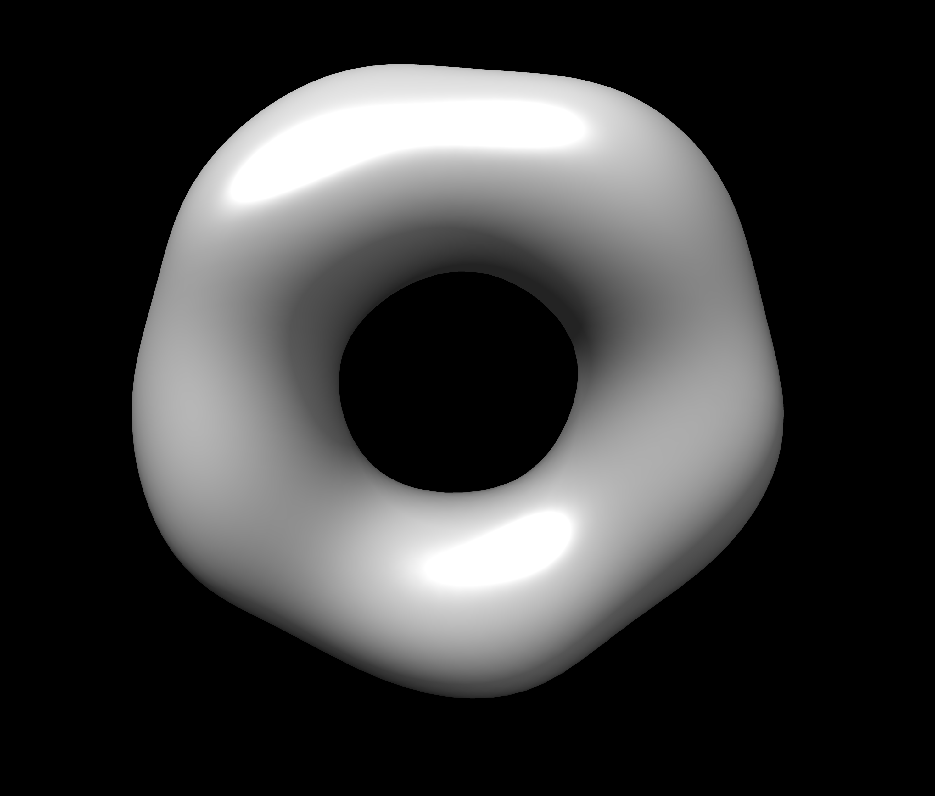
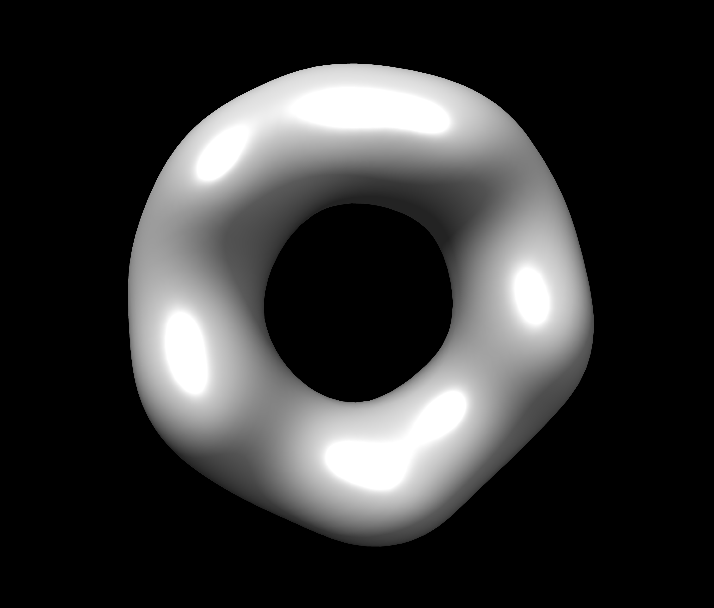
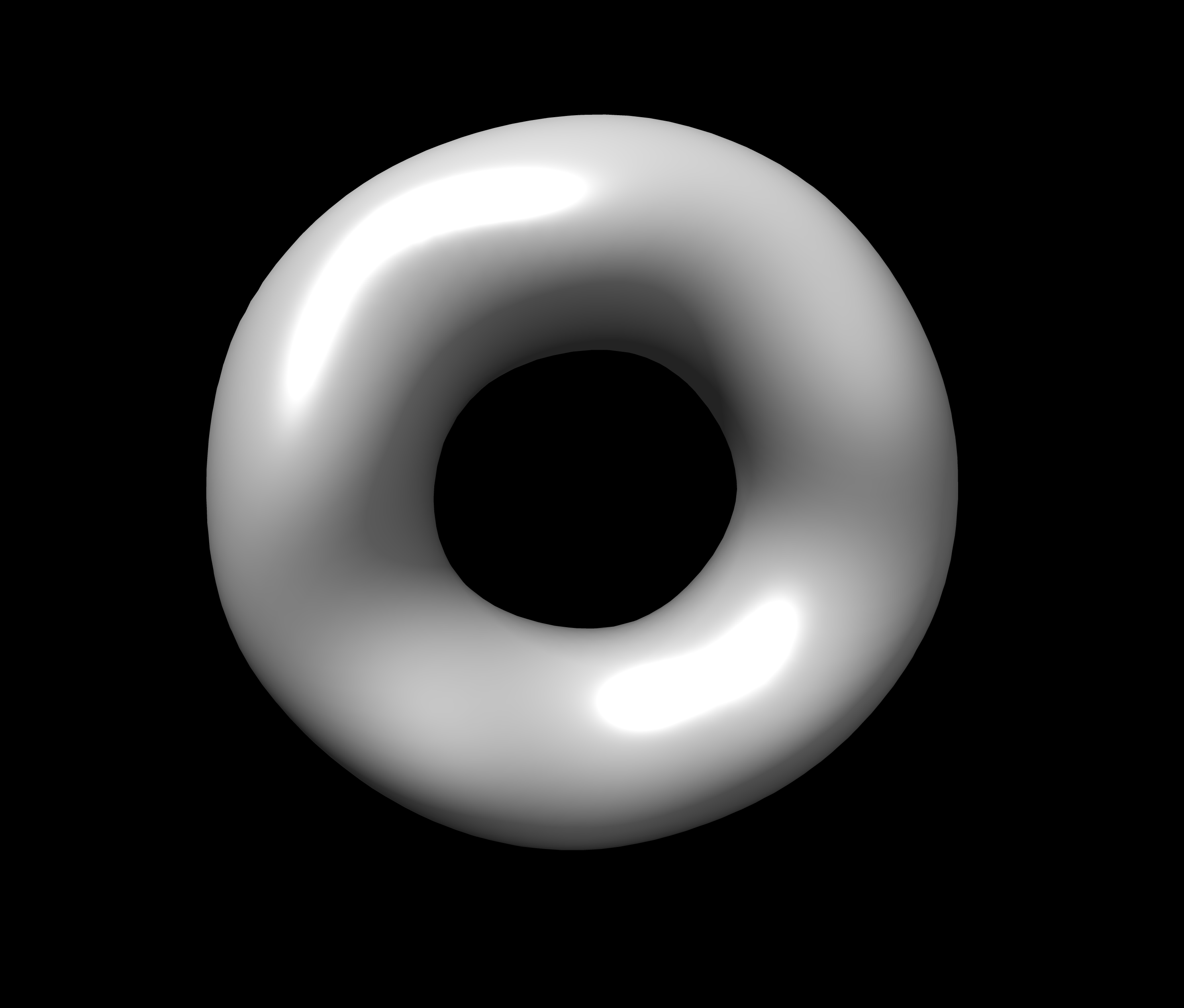
A ccp4 file is generated for each returned model. And models within the same cluster are averaged to a map. You can use chimera to view the models. Here gives the images of the top 3 models, from left to right.
One can provide a pdb file and compare the returned models with it.
sastbx.shapeup target=2e2g_znk.iq rmax=50 pdb=2e2g.pdb
Now the output shows cc to the model given by the pdb file.
Rank PDB_code cc (to the given model or the first model):
 1   2ZCT  0.997
 2   2H66  0.955
 3   1QMV  0.983
 4   1UUL  0.980
 5   2PN8  0.981
 6   2FB5  0.858
 7   1E2Y  0.956
 8   1J93  0.946
 9   1U3D  0.921
10   2OB9  0.948
Similarity of the returned models to the target is implied by the high values of cc.
Compare the average_model(ave_1.ccp4, left) to the pdb file provided (2e2g.pdb, right):

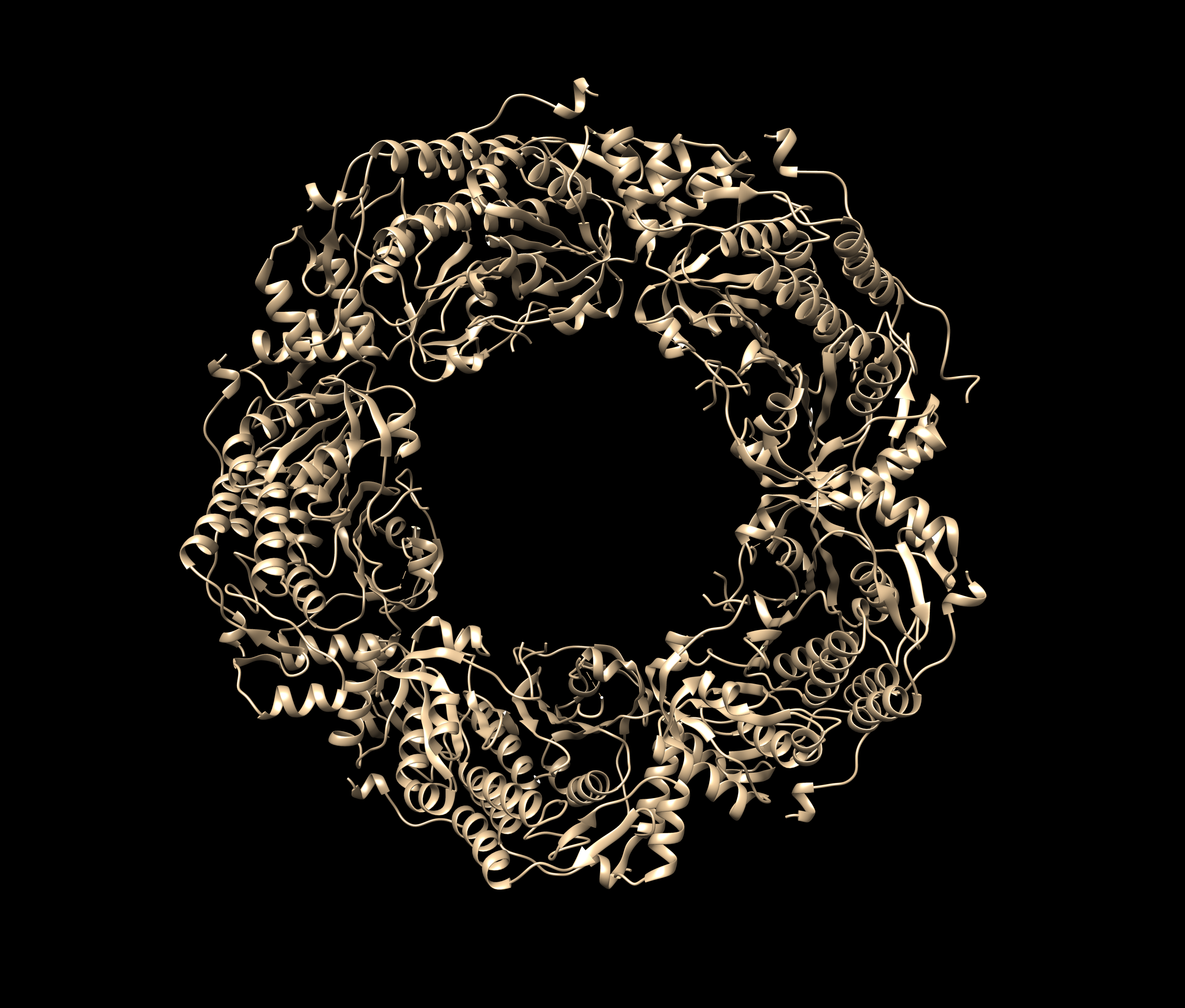
Rmax: estimated vs PDB 74.1502812526 72.9867447533